Second Problem Set: more problems

Differental Equation Video Clip Problems:
Master List Problem #'s from Boyce $\bullet$ DiPrima.

1.1

In Problem 6 draw a direction field for the given differential equation. Based on the direction field, determine the behavior of $y$ as $t \rightarrow \infty$. If this behavior depends on the initial value of $y$ at $t=0$, describe this dependency.

6. $y^{\prime} = y +2$

15. A pond initially contains 1,000,000 gal of water and an unknown amount of an undersirable chemical. Water containing 0.01 gram of this chemical per gallon flows into the pond at a rate of 300 gal/min. The mixture flows out at the same rate so the amount of water in the pond remains constant. Assume that the chemical is uniformly distributed throughout the pond.

(a) Write a differential equation whose solution is the amount of the chemical in the pond at any time.

(b) How much of the chemical will be in the pond after a very long time? Does this limiting amount depend on the amount that was present initially?

1.2

In Problem 1.(a) solve the following initial value problem and plot the solutions for several values of $y_0$. Then describe in a few words how the solutions resemble, and differ from, each other.

1.(a) ; $dy/dt = - y + 5, \qquad y(0) = y_0$

1.3

In Problem 1 determine the order of the given differential equaiton; also state whether the equation is linear or nonlinear.

1. $$t^2\frac{d^2 y}{dt^2} + t\frac{dy}{dt} + 2y = \mbox{sin} t$$

In Problem 11 verify that the given function or function is a solution of differential equations.

11. $2t^2y^{\prime\prime} + 3ty^{\prime} - y = 0,\quad t > 0;\qquad y(t) = t^{1/2}, \quad y_2(t) = t^{-1}$

In Problem 19 determine the values of $r$ for which the given differential equation has solutions of the form $y = e^{rt}$.

19. $r^2y^{\prime\prime} + 4ty^{\prime} + 2y = 0$

2.1 - In Problem 10:

(a) Draw a direction field for the given differential equation.

(b) Based on an inspection of the direction field, describe how solutions behave for large $t$.

(c) Find the general solution of the given differential equation and use it to determine how solutions behave as $t \rightarrow \infty$.

10. $$ty^{\prime} - y = t^2 e^{-t}$$

In Problem 13 find the solution of the given initial value problem.

13. $y^{\prime} - y = 2te^{2t}, \qquad y(0) = 1$

In Problem 22:

(a) Draw a direction field for the given differential equation. How do solutions appear to behave as $t$ becomes large? Does the behavior depend on the choice of the initial value $a$? Let $a_0$ be the value of $a$ for which the transition from one type of behavior to another occurs. Estimate the value of $a_0$.

(b) Solve the initial value problem and find the critical value $a_0$ exactly.

(c) Describe the behavior of the solution correponding to the initial value $a_0$.

22. $2y^{\prime} - y = e^{1/3}, \qquad y(0) = a$

2.2 - In Problem 9:

(a) Find the solution of the given initial value problem in explicit form.

(b) Plot the graph of the solution.

(c) Determine (at least approximately) the interval in which the solution is defined.

9. $y^{\prime} = (1 - 2x)y^2, \qquad y(0) = - 1/6$

22. Solve the initial value problem

$$y^{\prime} = 3x^2/(3y^2 - 4), \qquad y(1) = 0$$

and determine the interval in which the solution is valid. Hint: To find the interval of definition, look for points where the integral curve has a vertical tangent.

24. Solve the initial value problem

$$y^{\prime} = (2 - e^{x})/(3 + 2y), \qquad y(0) = 0$$

2.3

3. A tank originally contains 100 gal of fresh water. Then water containing $\frac{1}{2}$ lb of salt per gallon is poured into the tank at a rate of 2 gal/min, and the mixture is allowed to leave at the same rate. After 10 min the process is stopped, and fresh water is poured into the tank at a rate of 2 gal/min, with the mixture again leaving at the same rate. Find the amount of salt in the tank at the end of an additional 10 min.

10. A home buyer can afford to spend no more that $800/month on mortgage payments. Suppose that the interest rate is 9% and that the term of the mortgage is 20 years. Assume that interest is compounded continuously and that payments are also made continuously.

(a) Determine the maximum amount that this buyer can afford to borrow.

(b) Determine the total interest paid during the term of the mortgage.

2.5

Problem 3 involves equation of the form $dy/dt = f(y)$. Sketch the graph of $f(y)$ versus $y$, determine the critical (equilibrium) points, and classify each one as asymptotically stable or unstable.

3. $dy/dt = y(y -1)(y - 2), \qquad y_0 \geq 0$

Problem 9 involves equation of the form $dy/dt = f(y)$. Sketch the graph of $f(y)$ versus $y$, determine the critical (equilibrium) points, and classify each one as asymptotically stable, unstable, or semistable (see Problem 7).

Problem 7 Semistable Equlibrium Solutions. Sometimes a constant equilibrium solution has the property that solutions lying on one side of the equilibrium solution tend to approach it, whereas solutions lying on the other side depart from it (see Figure 2.5.10). In this case the equilibrium solution is said to be semistable.

(a) Consider the equation

$$dy/dt = k(1 - y)^2,$$

where $k$ is a positive constant. Show that $y = 1$ is the only critical point, with the corresponding equilibrium solution $\phi(t)=1$.

(b) Sketch $f(y)$ versus $y$. Show that $y$ is increasing as a function of $t$ for $y < 1$ and also for $y > 1$. Thus solutions below the equilibrium solution approach it, while those above it grow farther away. Therefore $\phi(t)=1$ is semistable.

FIGURE 2.5.10 In both cases the equilibrium solution $\phi (t) = k$ is semistable. $(a) dy/dt \leq 0$; ; (b)$dy/dt \leq 0$.

(c) Solve Eq. (i) subject to initial condition $y(0) = y_0$ and confirm the conclusions reach in part (b).

In Problem 9 involve equations of the form $dy/dt = f(y)$. Sketch the graph of $f(y)$ versus $y$, determine the critical (equilibrium) points, and classify each one as asymptotically stable, unstable, or semistable (see Problem 7).

9. $dy/dt = y^2(y^2 - 1), \qquad -\infty < y_0 < \infty$

18. A pond forms as water collects in a conical depression of radius $a$ and depth $h$. Suppose that water flows in at a constant rate $k$ and is lost through evaporation at a rate proportional to the surface.

(a) Show that the volume $V(t)$ of water in the pond at time $t$ satisfies the differential equation

$$dV/dt = k - \alpha\pi(3a/\pi h)^{2/3}V^{2/3},$$

where $\alpha$ is the coefficient of evaporation.

(b) Find the equilibrium depth of water in the pond. Is the equilibrium asymptotically stable?

(c) Find a condition that must be satisfied if the pond is not to overflow.

3.1

In Problem 9 find the solution of the given initial value problem. Sketch the graph of the solution and describe its behavior as $t$ increases.

9. $y^{\prime\prime} + y^{\prime} - 2y = 0, \qquad y(0) = 1, \quad y^{\prime}(0) = 1$

17. Find a differential equation whose general solution is $y= c_1 e^{2t} + c_2 e^{-3t}$.

21. Solve the initial value problem $y^{\prime\prime} - y^{\prime} - 2y = 0, ; ; y(0) = \alpha, ; ; y^{\prime}(0) = 2$. Then find $\alpha$ so that the solution approaches zero as $t \rightarrow \infty$.

3.2

In Problem 12 determine the longest interval in which the given initial value problem is certain to have a unique twice differentiable solution. Do not attempt to find the solution.

12. $(x - 2)y^{\prime\prime} + y^{\prime} + (x - 2)(\tan x)y = 0, \qquad y(3) = 1, \quad y^{\prime}(3) = 2$.

18. If the Wronskian $W$ of $f$ and $g$ is $t^2 e^t$, and if $f(t) = t$, find $g(t)$.

In Problem 25 verify that the functions $y_1$ and $y_2$ are solutions of the given differential equation. Do they constitute a fundamental set of solutions?

25. $x^2 y^{\prime\prime} - x(x+2)y^{\prime} + (x+2)y = 0, \quad x > 0, \qquad y_1(x) = x, \quad y_2(x) = xe^x$.

3.3

9. The Wronskian of two functions is $W(t) = t \sin^2 t$. Are the functions linearly independent or linearly dependent? Why?

In Problem 18 find the Wronskian of two solutions of the given differential equation without solving the equation.

18. $(1 - x^2)y^{\prime\prime} - 2xy^{\prime} + \alpha (\alpha + 1)y = 0, \qquad \mbox{Legendre's equation}$

In Problem 24 assume that $p$ and $q$ are continuous, and that the functions $y_1$ and $y_2$ are solutions of the differential equation $y^{\prime\prime} + p(t)y^{\prime} + q(t)y = 0$ on an open interval $I$.

24. Prove that if $y_1$ and $y_2$ are zero at the same point in $I$, then they cannot be a fundamental set of solutions on that interval.

3.4

In Problem 18 find the solution of the given initial value problem. Sketch the graph of the solution and describe its behavior for increasing $t$.

18. $y^{\prime\prime} + 4y^{\prime} + 5y = 0, \qquad y(0) = 1, \quad y^{\prime}(0) = 0$

27. Show that $W(e^{\lambda t} \cos \mu t, ; e^{\lambda t} \sin \mu t) = ue^{2\lambda t}.$

3.5

In Problem 1 find the general solution of the given differential equation.

1. $y^{\prime\prime} - 2y^{\prime} + y = 0$

18. Consider the initial value problem

$$9y^{\prime\prime} + 12y^{\prime} + 4y = 0, \qquad y(0) = \alpha > 0, \quad y^{\prime}(0) = - 1$$

(a) Solve the initial value problem.

(b) Find the critical value of $\alpha$ that separates solutions that become negative from those that are always positive.

In Problem 23 use the method of reduction of order to find a second solution of the given differential equation.

23. $t^2 y^{\prime\prime} - 4ty^{\prime} + 6y = 0, \quad t > 0; \qquad y_1(t) = t^2$

In Problem 36 use the method of Problem 33 to find a secomd indepenent solution of the given equation

36. $(x - 1)y^{\prime\prime} - xy^{\prime} + y = 0, \quad x > 1; \qquad y_1(x) = e^x$

3.6

In Problem 1, 3, and 7 find the general solution of the given differential equation.

1. $y^{\prime\prime} - 2y^{\prime} - 3y = 3e^{2t}$

3. $y^{\prime\prime} - 2y^{\prime} - 3y = -3te^{-t}$

7. $2y^{\prime\prime} + 3y^{\prime} +y = t^2 + 3 \sin t$

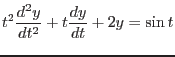
3.8

2. In Problem 2 determine $\omega_0, R,$ and $\delta$ so as to write the given expression in the form $u = R \cos(\omega_0 t - \delta)$.

2. $u = - \cos t + \sqrt{3} \sin t$

A. A mass weighing 32 lbs stretches a spring 2 ft at equilibrium. If the mass is pushed upward and released with an initial velocity of 4 ft/sec (downward), find $u(t)$. Also find $w_0, T, \delta, R$ and sketch the graph of $u(t)$.

B. A spring/mass system is modeled by the initial value problem: $2u^{\prime\prime} + \gamma u^{\prime} + 8u(0)$
$u(0) = 1, ; u^{\prime}(0) = 4$.

(a) Give a qualitatively accurate sketch of $u(t)$ for each indicated value of $\gamma$:

$$\gamma = 4, \quad \gamma = 7.9, \quad \gamma = 10, \quad \gamma = 1000.$$

(b) Find the value of $\gamma$ that makes the quasi-period $T_d$ 50% greater than the natural period.

10.1

In Problem 1 and 7 either solve the given boundary value problem or else show that it has no solution.

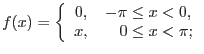
1. $y^{\prime\prime} + y = 0, \qquad y(0) = 0, \quad y^{\prime}(\pi) = 1$

7. $y^{\prime\prime} + 4y = \cos x, \qquad y(0) = 0, \quad y(\pi) = 0$

In Problem 11 find the eigenvalues and eigenfunctions of the given boundary value problem. Assume that all eigenvalues are real.

11. $y^{\prime\prime} + \lambda y = 0, \qquad y(0) = 0, \quad y^{\prime}(\pi) = 0$

10.2

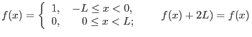
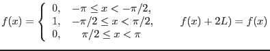
In Problems 14 and 16

(a) Sketch the graph of the given function for three periods.
(b) Find the Fourier series for the given function.

14. $f(x) = \left\{ \begin{array}{cc} 1, & -L \leq x < 0,\\ 0, & \quad0 \leq x < L; \end{array}\qquad f(x) + 2L) = f(x) \right.$

16. $f(x) = \left\{ \begin{array}{cc} x+1, & -1 \leq x < 0,\\ 1-x, & \quad 0 \leq x < 1; \end{array}\qquad f(x + 2) = f(x) \right.$

In Problem 19

(a) Sketch the graph of the given function for three periods.
(b) Find the Fourier series for the givenfunction.
(c) Plot $s_m(x)$ versus $x$ for $m$ = 5, 10, and 20.
(d) Describe how the Fourier series seems to be converging.

19. $f(x) = \left\{ \begin{array}{cc} -1, & -2 \leq x < 0,\\ \phantom{-}1, & \quad 0 \leq x < 2; \end{array}\qquad f(x + 4) = f(x) \right.$

10.3

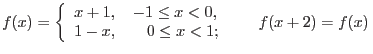
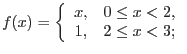
In Problems 2 and 5 assume that the given function is periodically extended outside the original interval.

(a) Find the Fourier series fore the extended function.
(b) Sketch the graph of the function to which the series converges for three periods.

2. $f(x) = \left\{ \begin{array}{cc} 0, & -\pi \leq x < 0,\\ x, & \quad 0 \leq x < \pi; \end{array}\right.$

5. $f(x) = \left\{ \begin{array}{cc} 0, & \!-\pi \leq x < -\pi/2,\\ 1, & -\pi/2 \l... ...pi/2,\\ 0, & \!\pi/2 \leq x < \pi \end{array}\qquad f(x) + 2L) = f(x) \right.$

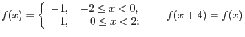
10.4

In Problems 1 and 2 determine whether the given function is even, odd, or neither.

1. $x^3 - 2x$

2. $x^3 - 2x + 1$

In Problem 7 a function $f$ is given on an interval of length $L$. In each case sketch the graphs of the even and odd extensions of $f$ of period $2L$.

7. $f(x) = \left\{ \begin{array}{cc} x, & 0 \leq x < 2,\\ 1, & 2 \leq x < 3; \end{array}\right.$

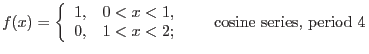
In Problem 15 find the required Fourier series for the given function and sketch the graph of the function to which the series converges over three periods.

15. $f(x) = \left\{ \begin{array}{cc} 1, & 0 < x < 1,\\ 0, & 1 < x < 2; \end{array}\qquad \mbox{cosine series, period 4} \right.$

10.5

In Problem 2 determine whether the method of separation of variables can be used to replace the given partial differential equation by a pair of ordinary differential equations.

2. $tu_{xx} + xu_{t} = 0$

A. Consider the two-point boundary value problem $X^{\prime\prime} + \sigma X = 0,\quad X^{\prime}(0) = X(L) = 0$. Find all eigenvalues $\sigma$ and corresponding eigenfunctions $X(x)$.

Consider the conduction of heat in a rod 40 cm in length whose ends are maintained at $0^{^{o}}$ for all $t>0$. Find an expression for the temperature $u(x,t)$ if the initial temperature distribution in the rod is the given function. Suppose that $\alpha^2 = 1$.

9. $u(x,0) = 50, \qquad 0 < x < 40$

10.6

In Problem 1 find the steady-state solution of the heat conductive equation $\alpha^2 u_{xx} = u$, that satisfies the given set of boundary conditions.

1. $u(0,t) = 10, \quad u(50,t) = 40$

9. Let an aluminum rod of length 20 cm be initially at the uniform temperature of 25$^{^{o}}$C. Suppose that at time $t=0$ the end $x=0$ is cooled to 0$^{^{o}}$C while the end $x = 20$ is heated to 60$^{^{o}}$C, and both are thereafter maintained at those temperatures.

(a) Find the temperature distributions in the rod at any time $t$.

(b) Plot the initial temperature distribution, the final (steady-state) temperature distribution, and the temperature distribution at two representative intermediate times on the same set of axes.

(c) Plot $u$ versus $t$ for $x=5$, 10, and 15.

7.1

In Problem 4 transform the given equation into a system of first order equations.

4. $u^{\prime\prime\prime\prime} - u = 0$

18. Consider the circuit shown in Figure 7.1.2. Let $I_1, I_2$, and $I_3$ be the current through the capacitor, resistor, and inductor, respectively. Likewise, let $V_1, V_2$, and $V_3$ be the corresponding voltage drops. The arrows denote the arbitrarily chosen directions in which currents and voltage drops will be taken to be positive.

(a) Applying Kirchhoff's second law to the upper loop in the circuit, show that

$$V_1 - V_2 = 0. \hspace*{2.0in} (i)$$

In a similar way, show that

$$V_2 - V_3 = 0. \hspace*{2.0in} (ii)$$

(b) Applying Kirchhoff's first law to either node in the circuit, show that

$$I_1 + I_2 + I_3 = 0. \hspace*{1.75in} (iii)$$

(c) Use the current-voltage relation through each element in the circuit to obtain the equations

$$CV^{\prime}_1 = I_1, \qquad V_2 = RI_2, \qquad LI^{\prime}_3 = V_3. \hspace*{.20in} (iv)$$

(d) Eliminate $V_2, V_3, I_1$, and $I_2$ among Eqs. (i) through (iv) to obtain

$$CV^{\prime}_1 = -1_3 - \frac{V_1}{R}, \qquad LI^{\prime}_3 = V_1. \hspace*{.70in} (v)$$

Observe that if we omit the subscripts in Eqs. (v), then we have the system (2) of the text.

7.2

1. If A = $\left( \begin{array}{ccc} \phantom{-}1 & -2 & \phantom{-}0\\ \phantom{-}3 & \phantom{-}2 & -1\\ -2 & \phantom{-}1 & \phantom{-}3 \end{array}\right)$ and B = $\left( \begin{array}{ccc} \phantom{-}4 & -2 & \phantom{-}3\\ -1 & \phantom{-}5 & \phantom{-}0\\ \phantom{-}6 & \phantom{-}1 & \phantom{-}2 \end{array}\right),$ find

(a) 2A + B (b) A $-$ 4B

(c) AB (d) BA

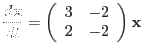
In Problem 22 verify that the given vector satisfies the given differential equation

22. ${\bf {x}}^{\prime} = \left( \begin{array}{cc} 3 & -2\\ 2 & -2 \end{array}\righ... ...x}, \qquad {\bf {x}} = \left( \begin{array}{c} 4\\ 2 \end{array}\right) e^{2t}$

7.3

In Problem 4 either solve the given set of equations, or else show that there is no solution.

4. $\begin{array}{ccccc} x_1 &+& 2x_2 &-& x_3 = 0 [5pt] 2x_1 &+& x_2 &+& x_3 = 0 [5pt] x_1 &-& x_2 &+& 2x_3 = 0 \end{array}$

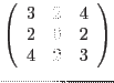
In Problem 7. determine whether the given set of vectors is linearly independent. If linearly dependent, find a linear relation among them. The vectors are written as row vectors to save space, but may be considered as column vectors; that is, the transposes of the given vectors may be used instead of the vectors themselves.

7. ${\bf {x}}^{(1)} = (2, 1, 0), \qquad {\bf {x}}^{(2)} = (0, 1, 0), \qquad {\bf {x}}^{(3)} = (-1, 2, 0)$

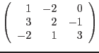
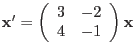
In Problem 15 find all eigenvalues and eigenvectors of the given matrix.

15. $\left( \begin{array}{cc} 5 & -1\\ 3 & \phantom{-}1 \end{array}\right)$

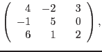
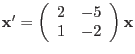
In Problem 24 find all eigenvalues and eigenvectors of the given matrix.

24. $\left( \begin{array}{ccc} 3 & 2 & 4\\ 2 & 0 & 2\\ 4 & 2 & 3 \end{array}\right)$

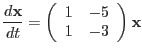
7.5

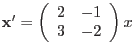
In Problem 3 and 5 find the general solution of the given system of equations and describe the behavior of the solution as $t \rightarrow \infty$. Also draw a direction field and plot a few trajectories of the system.

3. ${\bf {x}}^{\prime} = \left( \begin{array}{cc} 2 & -1\\ 3 & -2 \end{array}\right)x$

5. ${\bf {x}}^{\prime} = \left( \begin{array}{cc} -2 & \phantom{-}1\\ \phantom{-}1 & -2 \end{array}\right)x$

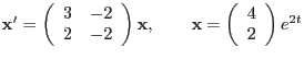
In Problem 15 solve the given initial value problem. Describe the behavior of the solution as $t \rightarrow \infty$.

15. ${\bf {x}}^{\prime} = \left( \begin{array}{cc} 5 & -1\\ 3 & \phantom{-}1 \end{a... ...d {\bf {x}}(0) = \left( \begin{array}{c} \phantom{-}2\\ -1 \end{array}\right)$

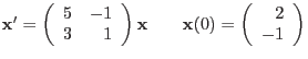
In Problem 27 the eigenvalues and eigenvectors of a matrix ${\bf {A}}$ is given. Consider the corresponding system ${\bf {x}}^{\prime} = {\bf {Ax}}$.

(a) Sketch a phase portrait of the system.

(b) Sketch the trajectory passing through the initial point (2, 3).

(c) For the trajectory in part (b) sketch the graphs of $x_1$ versus $t$ and of $x_2$ versus $t$ on the same set of axes.

27. $r_1 = 1, \quad {\bf {\xi}}^{(1)} = \left(\begin{array}{c}1 2\end{array}\right... ... {\bf {\xi}}^{(2)} = \left(\begin{array}{c}\phantom{-}1 -2\end{array}\right)$

7.6

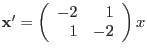
In Problem 1 and 3 express the general solution of the given system of equations in terms of real-valued functions. Also draw a direction field, sketch a few of the trajectories, and describe the behavior of the solution as $t \rightarrow \infty$.

1. ${\bf {x}}^{\prime} = \left( \begin{array}{cc} 3 & -2\\ 4 & -1 \end{array}\right){\bf {x}}$

3. ${\bf {x}}^{\prime} = \left( \begin{array}{cc} 2 & -5\\ 1 & -2 \end{array}\right){\bf {x}}$

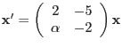
In Problem 15 the coefficient matrix contains a parameter $\alpha$. In this problem:

(a) Determine the eigenvalues in terms of $\alpha$.

(b) Find the critical value of values of $\alpha$ where the qualitative nature of the phase portrait for the system changes.

(c) Draw a phase portrait for a value of $\alpha$ slightly below, and for another value slightly above, each critical value.

15. ${\bf {x}}^{\prime} = \left( \begin{array}{cc} 2 & -5\\ \alpha & -2 \end{array}\right){\bf {x}}$

9.1

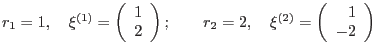
For each of the systems in Problems 1 and 5:

(a) Find the eigenvalues and eigenvectors.

(b) Classify the critical point (0, 0) as to type and determine whether it is stable, asymptotically stable, or unstable.

(c) Sketch several trajectories in the phase plane and also sketch some typical graphs of $x_1$ versus $t$.

(d) Use a computer to plot accurately the curves requested in part (c).

1. $$\frac{d{\bf {x}}}{dt} = \left( \begin{array}{cc} 3 & -2\\ 2 & -2 \end{array}\right){\bf {x}}$$

5. $$\frac{d{\bf {x}}}{dt} = \left( \begin{array}{cc} 1 & -5\\ 1 & -3 \end{array}\right){\bf {x}}$$

9.2

In Problem 1 sketch the trajectory corresponding to the solution satisfying the specified initial conditions, and indicate the direction of motion for increasing $t$.

1. $dx/dt = - x, \quad dy/dt = - 2y; \quad x(0) = 4, \quad y(0) = 2$

For each of the systems in Problem 5:

(a) Find all the critical points (equilibrium solutions).

(b) Use a computer to draw a direction field and phase portrait for the system.

(c) From the plot(s) in part (b) determine whether each critical point is asymptotically stable, stable, or unstable, and classify it as to type.

5. $dx/dt = x - xy, \qquad dy/dt = y + 2xy$ < A. Consider the autonomous system ; $$\frac{dx}{dt} = y, \qquad \displaystyle\frac{dy}{dt} = x^2 - x$$

(a) Find all critical points.

(b) Find an equation of the form $H(x,y) = c$ satisfied by solutions.

(c) Plot $H(x,y) = c$ for several $c$-values using MAPLE; indicate the direction of motion along trajectories.

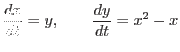
9.3

Problem 1 verify that (0, 0) is a critical point, show that the system is almost linear, and discuss the type and stability of the critical point (0, 0) by examining the corresponding linear system.

1. $dx/dt = x - y^2, \qquad dy/dt = x -2y + x^2$

In Problem 5:

(a) Determine all critical points of the given system of equations.

(b) Find the corresponding linear system near each critical point.

(c) Find the eigenvalues of each linear system. What conclusions can you then draw about the nonlinear system?

(d) Draw a phase portrait of the nonlinear system to confirm your conclusions, or to extend them in those cases where the linear system does not provide definite information about the nonlinear system.

5. $dx/dt = (2 + x)(y - x), \qquad dy/dt = (4 - x)(y + 1)$

17. Consider the autonomous system

$$dx/dt< = y, \qquad dy/dt = x + 2x^3.$$

(a) Show that the critical point (0, 0) is a saddle point.

(b) Sketch the trajectories for the corresponding linear system by integrating the equation for $dy/dx$. Show from the parametric form of the solution that the only trajectory on which $x \rightarrow 0, y \rightarrow 0$ as $t \rightarrow \infty$ is $y = - x$.

(c) Determine the trajectories for the nonlinear system by integrating the equation for $dy/dx$. Sketch the trajectories for the nonlinear system that correspond to $y = - x$ and $y = x$ for the linear system.