Next: Numerical Results.
Up: Differential Kinetic Equation
Previous: Derivation of Differential Quantum
Let us now rewrite the DQKE in the form:
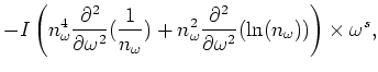
We can now use (3.11) to calculate the fluxes  and
and  in
terms of
in
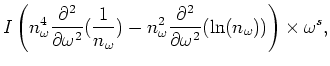
terms of  and its derivatives. We concentrate on the fermionic
case. There,
and its derivatives. We concentrate on the fermionic
case. There,
Let
us make a change of variables  and
and  .
.  are functions of
  and
and  , ``dot'' is used to denote
differentiation with respect to time, and ``prime'' with respect to
. Then
, ``dot'' is used to denote
differentiation with respect to time, and ``prime'' with respect to
. Then
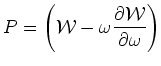
Since the stationary DQKE is a fourth order ODE,
its solutions will have four free parameters. Indeed, assume a steady
(equilibrium) state and integrate (4.9,4.11) twice to
get
where and are fluxes of
particle number and energy. For  , (4.12) trivially
gives
, (4.12) trivially
gives
the Fermi-Dirac distribution function.
Therefore we observe that the Fermi-Dirac distribution
function corresponds to a zero flux solution of the kinetic
equation, consistent with our findings of the previous section.
Next: Numerical Results.
Up: Differential Kinetic Equation
Previous: Derivation of Differential Quantum
Dr Yuri V Lvov
2007-01-31
![$\displaystyle \frac{\partial^2}{\partial \omega ^2} {\cal W}[n_\omega ],$](img227.png)