


Next: Conclusions
Up: General case of waves
Previous: Theorem
Bose-Einstein Condensate (BEC) is a state of matter that arises in
dilute gases with large number of particles at very low
temperatures [19,20,21,22,23,24]. BEC
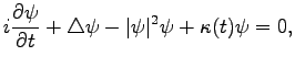
can be described by the Nonlinear Schrödinger equation (also known as
Gross-Pitaevskii equation [25]). Here, we apply the
theorem to this well studied model. The evolution of the state
function  is described by the following equation
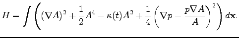
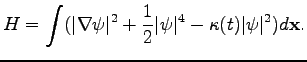
with a corresponding Hamiltonian
The term
 is introduced for convenience as will become
clear later. Following [7], let us consider the
amplitude-phase representation of the order parameter
:
is introduced for convenience as will become
clear later. Following [7], let us consider the
amplitude-phase representation of the order parameter
:
Now, we introduce Hamiltonian momentum
 |
|
|
(77) |
and rewrite Eq. (87) in terms of new canonical variables  and
and
 as
as
where
 |
|
|
(79) |
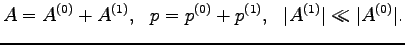
Let us consider weak perturbations on background of a strong
condensate,
 |
|
|
(80) |
We now choose
 which gives us
 . Substituting Eq. (90) into
Eq. (89) we have
. Substituting Eq. (90) into
Eq. (89) we have
where the subscripts denote the order of the term with respect to
perturbation amplitudes. Since in this paper we study the linear
dynamics, we only consider the quadratic part of the Hamiltonian
Here, we used the fact that the spatial derivative adds one order in
 and we neglected the terms of the order two and higher.
In order to apply the theorem to  we first transform to Fourier
space and then switch to normal variables. Let us denote
we first transform to Fourier
space and then switch to normal variables. Let us denote
 ,
,
 and
and
 . We have
  and
and
 . Transforming
into Fourier space we obtain
. Transforming
into Fourier space we obtain
where we used the following simplified notations:
 ,
,
 and subscript
 . Next, we switch
to normal variables using the transformation
. Next, we switch
to normal variables using the transformation
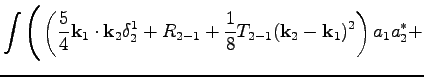
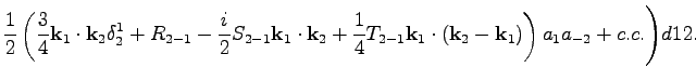
In normal variables,
reads
The only part of the coefficient in the second parenthesis we are
interested in is the one that satisfies Eq. (65):
Since  and
and  are slowly varying functions of
 , so
are
, so
are
 ,
,
 and
and
 . Therefore, their Fourier transforms
are peaked around zero making the terms proportional to
. Therefore, their Fourier transforms
are peaked around zero making the terms proportional to
 of the second order in
, which can
be neglected. Finally, we can write down the Hamiltonian in the form
given in Eq. (4)
of the second order in
, which can
be neglected. Finally, we can write down the Hamiltonian in the form
given in Eq. (4)
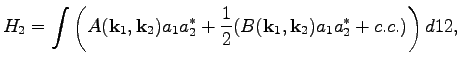 |
|
|
(82) |
where
In terms of window transformations, which we denote here as  the
Hamiltonian reads
the
Hamiltonian reads
where
Up to the first order in
, we have
Here,  is an even function of
 which means that
 and
and
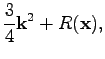
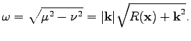
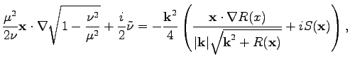
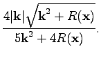
 . Then, the position dependent frequency of the small
perturbations in the presence of the condensate becomes
. Then, the position dependent frequency of the small
perturbations in the presence of the condensate becomes
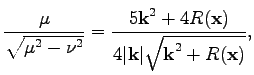
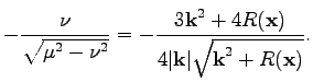
Bogolyubov's transformation,
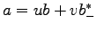 , is given by the following
coefficients
, is given by the following
coefficients
In terms of variables  the Hamiltonian takes the following form
where
Finally, we perform the near-identity transformation
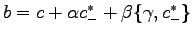 where
where
The resulting Hamiltonian attains the canonical form (5).
Next: Conclusions
Up: General case of waves
Previous: Theorem
Dr Yuri V Lvov
2008-07-08


![$\displaystyle H_f=\int a (\mu-\textbf{x}\cdot\nabla\mu+i\{\mu,\cdot\})a^*d\text...
...xtbf{x}\cdot\nabla\lambda+i\{\lambda,\cdot\}]a_{-}d\textbf{k}d\textbf{x}+c.c.],$](img383.png)


![$\displaystyle \int b(\omega-\textbf{x}\cdot\nabla_{\textbf{x}}\omega+i\{\omega,...
...ev}^2}{\nu}\left\{\varphi,b_-\right\}\right]d\textbf{k}d\textbf{x}+c.c.\right),$](img399.png)