Next: Resonance width
Up: Interactions of renormalized waves
Previous: Dispersion relation and resonances
Self-consistency approach to frequency renormalization
We now turn to the discussion of how
the trivial resonances give rise to the dispersion renormalization.
This question was examined in [12] before. There, it was
shown that the renormalization of the linear dispersion of the
 -FPU chain arises due to the collective effect of the
nonlinearity. In particular, the trivial resonant interactions of
type
-FPU chain arises due to the collective effect of the
nonlinearity. In particular, the trivial resonant interactions of
type
 , i.e., the solutions of Eq. (41),
enhance the linear dispersion (the renormalized dispersion relation
takes the form
, i.e., the solutions of Eq. (41),
enhance the linear dispersion (the renormalized dispersion relation
takes the form
 with
with  ), and effectively
weaken the nonlinear interactions. Here, we further address this
issue and present a self-consistency argument to arrive at an
approximation for the renormalization factor
), and effectively
weaken the nonlinear interactions. Here, we further address this
issue and present a self-consistency argument to arrive at an
approximation for the renormalization factor  . As it was
mentioned above, the contribution of the non-resonant terms have a
vanishing long time effect to the statistical properties of the
system, therefore, in our self-consistent approach, we ignore these
non-resonant terms. By removing the non-resonant terms and using the
canonical transformation
. As it was
mentioned above, the contribution of the non-resonant terms have a
vanishing long time effect to the statistical properties of the
system, therefore, in our self-consistent approach, we ignore these
non-resonant terms. By removing the non-resonant terms and using the
canonical transformation
 |
|
|
(45) |
where  is a
factor to be determined, we arrive at a simplified effective
Hamiltonian from Eq. (32) for the finite -FPU system
is a
factor to be determined, we arrive at a simplified effective
Hamiltonian from Eq. (32) for the finite -FPU system
The ``off-diagonal'' quadratic terms
 from
Eq. (32) are not present in Eq. (46), since
from
Eq. (32) are not present in Eq. (46), since
 are chosen so that
 (see
Section II). The contribution of the
trivial resonances in
(see
Section II). The contribution of the
trivial resonances in
 is
is
 |
|
|
(47) |
which can be ``linearized'' in the sense that averaging the
coefficient in front of
 in
in
 gives rise to
a quadratic form
gives rise to
a quadratic form
Note that the subscript  in
in
 emphasizes the
fact that
now can be viewed as a Hamiltonian for the
free waves with the familiar effective linear dispersion
emphasizes the
fact that
now can be viewed as a Hamiltonian for the
free waves with the familiar effective linear dispersion
 [12,5].
This linearization is essentially a mean-field approximation, since
the long-time average of trivial resonances in Eq. (47)
is approximated by the interaction of waves
with background
waves
[12,5].
This linearization is essentially a mean-field approximation, since
the long-time average of trivial resonances in Eq. (47)
is approximated by the interaction of waves
with background
waves
 . The self consistency condition, which
determines , can be imposed as follows: the quadratic
part of the Hamiltonian (46), combined with the
``linearized'' quadratic part,
, of the quartic
, should be equal to an effective quadratic
Hamiltonian
. The self consistency condition, which
determines , can be imposed as follows: the quadratic
part of the Hamiltonian (46), combined with the
``linearized'' quadratic part,
, of the quartic
, should be equal to an effective quadratic
Hamiltonian
 for the
renormalized waves, i.e.,
for the
renormalized waves, i.e.,
where
 is the renormalized linear dispersion, which is
used in the definition of our renormalized wave, Eq. (45),
and
is the renormalized linear dispersion, which is
used in the definition of our renormalized wave, Eq. (45),
and
 . Equating the coefficients of
 on both sides for every wave number
  yields
where use is made of
Eq. (33). After algebraic simplification, we have the
following equation for
 |
|
|
(48) |
Using the property (21) of the renormalized normal
variables
, we find the following dependence of
 on ,
on ,
 |
|
|
(49) |
Combining Eqs. (49) and (50) leads to
 |
|
|
(50) |
where
The only physically relevant solution of
Eq. (51) is
 |
|
|
(51) |
The
constants  and
and  can be easily derived using the Gibbs measure.
Next, we compare the renormalization factor [Eq. (25)]
with its approximation [Eq. (52)] from the
self-consistency argument. In Appendix A, we study in
detail the behavior of both and in the two
limiting cases, i.e., when nonlinearity is small (
 with fixed total energy
  ), and when nonlinearity is large
(
), and when nonlinearity is large
(
 with fixed total energy ). As is shown
in Appendix A, for the case of small nonlinearity, both
and have the same asymptotic behavior in the
first order of the small parameter ,
with fixed total energy ). As is shown
in Appendix A, for the case of small nonlinearity, both
and have the same asymptotic behavior in the
first order of the small parameter ,
Moreover,
in the case of strong nonlinearity
, both
and scale as
 , i.e.,
 |
|
|
(53) |
(see
Appendix A for details). Note that, in [12],
we numerically obtained the scaling
 , which
differs from the exact analytical result (54) due to
statistical errors in the numerical estimate of the power.
, which
differs from the exact analytical result (54) due to
statistical errors in the numerical estimate of the power.
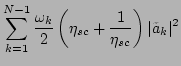
Figure 5:
The renormalization factor as a function of the
nonlinearity strength for small values of . The
renormalization factor [Eq. (25)] is shown with the
solid line. The approximation [Eq. (52)](via
the self-consistency argument) is depicted with diamonds connected
with the dashed line. The small- limit
[Eq. (53)] is shown with the solid circles connected
with the dotted line. Note that, abscissa is of logarithmic scale.
Inset: The renormalization factor as a function of the nonlinearity
strength for large values of . The renormalization
factor [Eq. (25)] is shown with the solid line.
[Eq.(52)] is depicted with diamonds connected
with the dashed line. The large- scaling
[Eq. (54)] is shown with the dashed-dotted line. Note
that, the plot is of log-log scale with base 10.
![\includegraphics[width=3in, height=3in]{eta_in}](img296.png) |
In Fig. 5, we plot the renormalization factor
and its approximation for the case of small
nonlinearity for the system with  particles and total
energy
particles and total
energy  . The solid line shows computed via
Eq. (25), the diamonds with the dashed line represent the
approximation via Eq. (52), and the solid circles with
the dotted line correspond to the small-
limit (53). In Fig. 5 (inset), we
plot the renormalization factor and its approximation
for the case of large nonlinearity for the
system with particles and total energy . The solid
line shows computed via Eq. (25), the diamonds with
the dashed line represent the approximation via Eq. (52),
and the dashed-dotted line correspond to the large-
scaling (54). Figure 5 shows good
agreement between the renormalization factor and its
approximation from the self consistency argument for a
wide range of nonlinearity, from
. The solid line shows computed via
Eq. (25), the diamonds with the dashed line represent the
approximation via Eq. (52), and the solid circles with
the dotted line correspond to the small-
limit (53). In Fig. 5 (inset), we
plot the renormalization factor and its approximation
for the case of large nonlinearity for the
system with particles and total energy . The solid
line shows computed via Eq. (25), the diamonds with
the dashed line represent the approximation via Eq. (52),
and the dashed-dotted line correspond to the large-
scaling (54). Figure 5 shows good
agreement between the renormalization factor and its
approximation from the self consistency argument for a
wide range of nonlinearity, from
 to
to
 . This agreement demonstrates, that (i) the effect of the
linear dispersion renormalization, indeed, arises mainly from the
trivial four-wave resonant interactions, and (ii) our
self-consistency, mean-field argument is not restricted to small
nonlinearity.
. This agreement demonstrates, that (i) the effect of the
linear dispersion renormalization, indeed, arises mainly from the
trivial four-wave resonant interactions, and (ii) our
self-consistency, mean-field argument is not restricted to small
nonlinearity.
Next: Resonance width
Up: Interactions of renormalized waves
Previous: Dispersion relation and resonances
Dr Yuri V Lvov
2007-04-11